Wednesday, 11 July 2012

Optimizing Writes in HBase

I've written a few times about our work to improve the scanning performance of our cluster (parts 1, 2, and 3) since our highest priority for HBase is being able to serve requests for downloads of occurrence records (which require a full table scan). But now that the scanning is working nicely we need to start writing new records into our occurrence table as well as cleaning raw data and interpreting it into something more useful for the users of our data portal. That processing is built as Hive queries that read from and write back to the same HBase table. And while it was working fine on small test datasets, it all blew up once I moved the process to the full dataset. Here's what happened and how we fixed it. Note that we're using CDH3u3, with the addition of Hive 0.9.0, which we patched to support HBase 0.90.4.

The problem

Our processing is Hive queries which run as Hadoop MapReduce jobs. When the mappers were running they would eventually fail (repeatedly, ultimately killing the job) with an error that looks like this:

java.io.IOException: org.apache.hadoop.hbase.client.ScannerTimeoutException: 63882ms passed since the last invocation, timeout is currently set to 60000

We did some digging and found that this exception happens when the scanner's next() method hasn't been called within the timeout limit. We simplified our test case by reproducing this same error when doing a simple CopyTable operation (the one that ships with HBase), and again using Hive to do select overwrite table A select * from table B. In both cases mappers are assigned a split to scan based on TableInputFormat (just like our Hive jobs), and as they scan they simply put the record out to the new table. Something is holding up the loop as it tries to put, preventing it from calling next(), and thereby triggering the timeout exception.

The logs

First stop - the logs. The regionservers are littered with lines like the following:

WARN org.apache.hadoop.hbase.regionserver.MemStoreFlusher: Region occurrence,\x17\xF1o\x9C,1340981109494.ecb85155563c6614e5448c7d700b909e. has too many store files; delaying flush up to 90000ms
INFO org.apache.hadoop.hbase.regionserver.HRegion: Blocking updates for 'IPC Server handler 7 on 60020' on region occurrence,\x17\xF1o\x9C,1340981109494.ecb85155563c6614e5448c7d700b909e.: memstore size 128.2m is >= than blocking 128.0m size

Well, blocking updates sure sounds like the kind of thing that would prevent a loop from writing more puts and dutifully calling next(). After a little more digging (and testing with a variety of hbase.client.scanner.caching values, including 1) we concluded that yes, this was the problem, but why was it happening?

Why it blocks

It blocks because the memstore has hit what I'll call the "memstore blocking limit" which is controlled by the setting hbase.hregion.memstore.flush.size * hbase.hregion.memstore.block.multiplier, which by default are 64MB and 2 respectively. Normally the memstore should flush when it reaches the flush.size, but in this case it reaches 128MB because it's not allowed to flush due to too many store files (the first log line). The definition of "too many storefiles" is in turn a setting, namely hbase.hstore.blockingStoreFiles (default 7). A new store file is created every time the memstore flushes, and their number is reduced by compacting them into fewer, bigger storefiles during minor and major compactions. By default, compactions will only start if there are at least hbase.hstore.compactionThreshold (default 3) store files, and won't compact more than hbase.hstore.compaction.max (default 7) in a single compaction. And regardless of what you set flush.size to, the memstore will always flush if all memstores in the regionserver combined are using too much heap.  The acceptable levels of heap usage are defined by hbase.regionserver.global.memstore.lowerLimit (default 0.35) and hbase.regionserver.global.memstore.upperLimit (default 0.4). There is a thread dedicated to flushing that wakes up regularly and checks these limits:

  • if the flush thread wakes up and memstores are greater than the lower limit it will start flushing (starting with current biggest memstore) until it gets below the limit.
  • if flush thread wakes up and memstores are greater than the upper limit it will block updates and start flushing until it gets under lower limit, when it unblocks updates.
Fortunately we didn't see blocking because of the upper heap limit - only the "memstore blocking limit" described earlier. But at this point we only knew the different dials we could turn.

Stopping the blocking

Our goal is to stop the blocking so that our mapper doesn't timeout, while at the same time not running out of memory on the regionserver. The most obvious problem is that we have too many storefiles, which appears to be a combination of producing too many of them and not compacting them fast enough. Note that we have a 6GB heap dedicated to HBase, but can't afford to take any more away from the co-resident Hadoop mappers and reducers.

We started by upping the memstore flush size - this will produce fewer but bigger storefiles on each flush:
  • first we tried 128MB with block multiplier still at 2. This still produced too many storefiles and caused the same blocking (maybe a little better than at 64MB)
  • then tried 256MB with multiplier of 4.  The logs and ganglia showed that the flushes were happening well before 256MB (still around 130MB) "due to global heap pressure" - a sign that total memstores were consuming too much heap. This meant we were still generating too many files and got the same blocking problem, but with the "memstore blocking limit" set to 1GB the memstore blocking happened much less often, and later in the process (still killed the mappers though)
We were now producing fewer storefiles, but they were still accumulating too quickly. From ganglia we also saw that the compaction queue and storefile counts were growing unbounded, which meant we'd hit the blocking limit again eventually. Next came trying to compact more files per compaction, hence raised compaction.max to 20, and this made little difference.

So how to reduce the number of storefiles? If we had fewer stores, we'd be creating fewer files and using up less heap for memstore, so next we increased the region size.  This meant increasing the setting hbase.hregion.max.filesize from its default of 256MB to 1.5G, and then rebuilding our table with fewer pre-split regions.  That resulted in about 75% fewer regions.

It was starting to look good - the number of "Blocking updates" log messages dropped to a handful per run, but it was still enough to affect one or two jobs to the point of them getting killed.  We tried upping the memstore.lowerLimit and upperLimit to 0.45 and 0.5 respectively, but again no joy.

Now what?

Things looked kind of grim. After endless poring over ganglia charts, we kept coming back to one unexplained blip that seemed to coincide with the start of the storefile explosion that eventually killed the jobs.
Figure 1: Average memstore flush size over time
At about the halfway point of the jobs the size of memstore flushes would spike and then gradually increase until the job died. Keep in mind that the chart shows averages, and it only took a few of those flushes to wait for storefiles long enough to fill to 1GB and then start the blocking that was our undoing. Back to the logs.

From the start of Figure 1 we can see that things appear to be going smoothly - the memstores are flushing at or just above 256MB, which means they have enough heap and are doing their jobs. From the logs we see the flushes happening fine, but there are regular lines like the following:
INFO org.apache.hadoop.hbase.regionserver.MemStoreFlusher: Under global heap pressure: Region uat_occurrence,\x06\x0E\xAC\x0F,1341574060728.ab7fed6ea92842941f97cb9384ec3d4b. has too many store files, but is 625.1m vs best flushable region's 278.2m. Choosing the bigger.
This isn't quite as bad as the "delaying flush" line, but it shows that we're on the limit of what our heap can handle. Then starting from around 12:20 we see more and more like the following:
WARN org.apache.hadoop.hbase.regionserver.MemStoreFlusher: Region uat_occurrence,"\x98=\x1C,1341567129447.a3a6557c609ad7fc38815fdcedca6c26. has too many store files; delaying flush up to 90000ms
and then to top it off:
INFO org.apache.hadoop.hbase.regionserver.wal.HLog: Too many hlogs: logs=35, maxlogs=32; forcing flush of 1 regions(s): ab7fed6ea92842941f97cb9384ec3d4b
INFO org.apache.hadoop.hbase.regionserver.MemStoreFlusher: Flush thread woke up with memory above low water.
So what we have is memstores initially being forced to flush because of minor heap pressure (adds storefiles faster than we can compact). Then we have memstores delaying flushes because of too many storefiles (memstores start getting bigger - our graph spike). Then the write ahead log (WAL) complains about too many of its logs, which forces a memstore flush (so that the WAL HLog can be safely discarded - this again adds storefiles).  And for good measure the flushing thread now wakes up, finds its out of heap, and starts attempting flushes, which just aggravates the problem (adding more storefiles to the pile). The failure doesn't happen immediately but we're past the point of no return - by about 13:00 the memstores are getting to the "memstore blocking limit" and our mappers die.

What's left?


Knowing what's going on in the memstore flush size analysis is comforting, but just reinforces what we already knew - the problem is too many storefiles. So what's left?  Raising the max number of storefiles, that's what! Every storefile in a store consumes resources (file handles, xceivers, heap for holding metadata), which is why it's limited to a maximum of a very modest 7 files by default. But for us this level of write load is rare - in normal operations we won't hit anything like this, and having the capacity to write a whole bunch of storefiles over short-ish, infrequent bursts is relatively safe, since we know our nightly major compaction will clean them up again (and thereby free up all those extra resources). Crank that maximum up to 200 and, finally, the process works!

Conclusion

Our problem was that our compactions couldn't keep up with all the storefiles we were creating. We tried turning all the different HBase dials to get the storefile/compaction process to work "like they're supposed to", but in the end the key for us was the hbase.hstore.blockingStoreFiles parameter which we set to 200, which is probably double what we actually needed but gives us buffer for our infrequent, larger write jobs. We additionally settled on larger (and therefore fewer) regions, and a somewhat bigger than default memstore. Here are the relevant pieces of our hbase-site.xml after all our testing:

  <!-- default is 256MB 268435456, this is 1.5GB -->
  <property>
    <name>hbase.hregion.max.filesize</name>
    <value>1610612736</value>
  </property>
  
  <!-- default is 2 -->
  <property>
    <name>hbase.hregion.memstore.block.multiplier</name>
    <value>4</value>
  </property>
  
  <!-- default is 64MB 67108864 -->
  <property>
    <name>hbase.hregion.memstore.flush.size</name>
    <value>134217728</value>
  </property>
  
  <!-- default is 7, should be at least 2x compactionThreshold -->
  <property>
    <name>hbase.hstore.blockingStoreFiles</name>
    <value>200</value>
  </property>

And finally, if our compactions were faster and/or more frequent, we might be able to keep up with our storefile creation. That doesn't look possible without multi-threaded compactions, but naturally those exist in newer versions of HBase (starting with 0.92 - HBASE-1476) so if you're having these problems, an upgrade might be in order. Indeed this is prompting us to consider an upgrade to CDH4.

Many thanks to Lars George, who helped us get through the "Now What?" phase by digging deep into the logs and the source to help us work out what was going on.

Monday, 18 June 2012

Launch of the Canadensys explorer

At Canadensys we already adopted and customized the IPT as our data repository. With the data of our network being served by the IPT, we have now built a tool to aggregate and explore these data. For an overview of how we built our network, see this presentation. The post below originally appeared on the Canadensys blog.

We are very pleased to announce the beta version of the Canadensys explorer. The tool allows you to explore, filter, visualize and download all the specimen records published through the Canadensys network.

The explorer currently aggregates nine published collections, comprising over half a million specimen records, with many more to come in the near future. All individual datasets are available on the Canadensys repository and via the Global Biodiversity Information Facility (GBIF) as well. The main functionalities of the explorer are listed below, but we encourage you to discover them for yourself instead. We hope it is intuitive. For the best user experience, please use an up-to-date version of your browser.

Happy exploring: http://data.canadensys.net/explorer

Functionalities

  • The explorer is a one page tool, limiting unnecessary navigation.
  • The default view shows all the data, allowing users to get an overview and explore immediately.
  • Data can be queried by using and combining filters.
  • Filters use smart suggestions, informing the user how often their search term occurs even before they search.
  • The exact number of results is displayed, including the number of georeferenced records.
  • The map view displays all georeferenced records for the current query, has different base layer options and can be zoomed in to any level.
  • Points on the map can be clicked for more information.
  • The table view displays a sortable preview of the records in the current query.
  • Records in the table can be clicked for more information in the same way as on the map.
  • The number of columns in the table responds to the screen width and can be controlled by the user in the display panel.
  • Data for the current query can be downloaded as a Darwin Core archive. There is no limit on the number of records that can be downloaded.
  • Users can download the data by providing their email address. Once the download package is generated, the user receives an email with a link to the data, information regarding the usage norms and a suggested citation.
  • The interface and emails are available in French and English.

As this is a beta version, you may encounter issues. Please report them by clicking the feedback button on the right, which will open a report form.

Technical details

The Canadensys explorer was developed using the following open source tools:

Tuesday, 12 June 2012

Taxonomic Trees in PostgreSQL

Taken aside pro parte synonyms taxonomic data follows a classic hierarchical tree structure. In relational databases such a tree is commonly represented by 3 models known as the adjacency list, the materialized path and the nested set model. There are many comparisons out there listing pros and cons, for example ON stackoverflow, the slides by Lorenzo Alberton or Bill Karwin or a postgres specific performance comparison between the adjacency model and a nested set.

Checklist Bank

At GBIF we use PostgreSQL to store taxonomic trees, which we refer to as checklists, in Checklist Bank. At the core there is a single table name_usage which contains records each representing a single taxon in the tree [note: in this post I am using the term taxon broadly covering both accepted taxa and synonyms]. It primarily uses the adjacency model with a single foreign key parent_fk which is null for the root elements of the tree. The simplified diagram of the main tables looks like this (actually there are some 20 extra fix width columns left out from name_usage here for simplicity):

For certain searches though an additional index is required. In particular listing all descendants of a taxon, i.e. all members of a subtree, is a common operation that would otherwise involve a recursive function or Common Table Expression. So far we have been using nested sets, but experiencing some badly performing queries lately I decided to do a quick evaluation of different options for Postgres:

  1. the ltree extension which implements a materialized path and provides many powerful operations.
  2. the intarray extension to manually manage a materialized path as an array of non null integers - the primary keys of the parent taxa.
  3. a simple varchar field holding the same materialized path
  4. the current nested set index using a lft and rgt integer column which is unique within a single taxonomy and therefore has to be combined with a checklist_key.

Test Environment

For the tests I am using the current Checklist Bank which contains 14,907,828 records in total spread across 107 checklists of varying size between 7 and 4.25 million records. I am querying the GBIF Backbone Taxonomy which is the largest checklist containing 4,251,163 records with 9 root taxa and a maximum depth of 11 levels. For the queries I have picked specific 2 taxa with different position in the taxonomic tree:

  1. 44 Vertebrata the class covering all vertebrates with approximately 84.100 species in this nub.
  2. 2684876 Abies the fir genus covering 167 species in this nub and exactly 609 descendants.
For most of our real queries we provide paging for larger results. I will therefore use a limit of 100 and offset of 0 for all queries below.

All tests are executed ON a 2Ghz i7 MacBook Pro with 8GB of memory running Postgres 9.1.1. All queries have been executed 3 times before EXPLAIN ANALYZE was used to get a rough idea ON how differently the various indices behave.

Creating the indices

In order to use the extensions these need to be compiled at installation time and enabled in the database. In Postgres 9.1 you can do the later by executing in psql:

  CREATE EXTENSION ltree;
  CREATE EXTENSION intarray;

The individual data types require different indices. We set up the following indices:

 # general indices
 CREATE INDEX nu_chkl_idx ON name_usage (checklist_fk);
 CREATE INDEX nu_parent_idx ON name_usage (parent_fk);
 # tree specifics
 CREATE INDEX nu_path_idx ON name_usage USING GIST (path);
 CREATE INDEX nu_mpath_idx ON name_usage USING GIN (mpath gin__int_ops);
 CREATE INDEX nu_mspath_idx ON name_usage (mspath);
 CREATE INDEX nu_ckl_lft_rgt_idx ON name_usage (checklist_fk, lft, rgt);

The ltree GIST and intarray GIN indices are rather expensive to create/maintain, but they are selected for best read performance.

Populating the indices

The data being imported into Checklist Bank comes with a parent-child relation, so parent_fk is populated already. For all other indices we have to populate the indices first.

ltree, intarray, string path

For all materialized paths I simply run the following SQL until no new updates happened:

# update root paths once
UPDATE name_usage u SET 
 path = text2ltree(cast(u.id as text)), 
 mspath=u.id, 
 mpath = array[u.id] 
WHERE u.parent_fk is null;
# update until no more records are updated
UPDATE name_usage u SET 
 path = p.path || text2ltree(cast(u.id as text)), 
 mspath=p.mspath || '.' || u.id, 
 mpath = p.mpath || array[u.id] 
FROM name_usage p 
WHERE u.parent_fk=p.id AND p.mspath is not null AND u.mspath is null;

nested sets

I've created 2 functions and one sequence to populate the lft/rgt indices for every checklist:

-- NESTED SET UTILITY FUNCTIONS
CREATE SEQUENCE name_usage_nestidx START 1;

CREATE FUNCTION update_nested_set_usage(integer) RETURNS BOOLEAN as $$
  BEGIN
    UPDATE name_usage set lft = nextval('name_usage_nestidx')-1 WHERE id=$1;
    PERFORM update_nested_set_usage(id) FROM usage WHERE parent_fk=$1 ORDER BY rank_fk, name_fk;;
    UPDATE name_usage set rgt = nextval('name_usage_nestidx')-1 WHERE id=$1;
    RETURN true;
  END
$$ LANGUAGE plpgsql;

CREATE FUNCTION build_nested_set_indices(integer) RETURNS BOOLEAN AS $$
BEGIN
  PERFORM setval('name_usage_nestidx', 1);
  PERFORM update_nested_set_usage(id) FROM usage WHERE parent_fk is null and checklist_fk=$1 ORDER BY rank_fk, name_fk;;
  RETURN true;
  END
$$ LANGUAGE plpgsql;

Query for Descendants

The queries return the first page with 100 records descendants

adjacency

A recursive postgres CTE query does the trick:

 WITH RECURSIVE d AS (
   SELECT id
    FROM name_usage
    WHERE id = 44
  UNION ALL
   SELECT c.id
    FROM d JOIN name_usage c ON c.parent_fk = d.id
 )
 SELECT * FROM d
  ORDER BY id
  LIMIT 100 OFFSET 0;
Query Plan: Abies
 Limit  (cost=74360.25..74360.50 rows=100 width=4) (actual time=7.306..7.337 rows=100 loops=1)
   CTE d
     ->  Recursive Union  (cost=0.00..72581.02 rows=30561 width=4) (actual time=0.041..6.017 rows=609 loops=1)
           ->  Index Scan using usage_pkey on name_usage  (cost=0.00..10.68 rows=1 width=4) (actual time=0.038..0.040 rows=1 loops=1)
                 Index Cond: (id = 2684876)
           ->  Nested Loop  (cost=0.00..7195.91 rows=3056 width=4) (actual time=0.240..1.393 rows=152 loops=4)
                 ->  WorkTable Scan on d  (cost=0.00..0.20 rows=10 width=4) (actual time=0.001..0.041 rows=152 loops=4)
                 ->  Index Scan using usage_parent_idx on name_usage c  (cost=0.00..715.75 rows=306 width=8) (actual time=0.006..0.008 rows=1 loops=609)
                       Index Cond: (parent_fk = d.id)
   ->  Sort  (cost=1779.24..1855.64 rows=30561 width=4) (actual time=7.304..7.316 rows=100 loops=1)
         Sort Key: d.id
         Sort Method: top-N heapsort  Memory: 29kB
         ->  CTE Scan on d  (cost=0.00..611.22 rows=30561 width=4) (actual time=0.046..6.678 rows=609 loops=1)
 Total runtime: 7.559 ms
Query Plan: Vertebrata
 Limit  (cost=74360.25..74360.50 rows=100 width=4) (actual time=2065.053..2065.080 rows=100 loops=1)
   CTE d
     ->  Recursive Union  (cost=0.00..72581.02 rows=30561 width=4) (actual time=0.105..1797.898 rows=264325 loops=1)
           ->  Index Scan using usage_pkey on name_usage  (cost=0.00..10.68 rows=1 width=4) (actual time=0.101..0.103 rows=1 loops=1)
                 Index Cond: (id = 44)
           ->  Nested Loop  (cost=0.00..7195.91 rows=3056 width=4) (actual time=0.915..182.695 rows=29369 loops=9)
                 ->  WorkTable Scan on d  (cost=0.00..0.20 rows=10 width=4) (actual time=0.007..8.056 rows=29369 loops=9)
                 ->  Index Scan using usage_parent_idx on name_usage c  (cost=0.00..715.75 rows=306 width=8) (actual time=0.004..0.005 rows=1 loops=264325)
                       Index Cond: (parent_fk = d.id)
   ->  Sort  (cost=1779.24..1855.64 rows=30561 width=4) (actual time=2065.050..2065.062 rows=100 loops=1)
         Sort Key: d.id
         Sort Method: top-N heapsort  Memory: 29kB
         ->  CTE Scan on d  (cost=0.00..611.22 rows=30561 width=4) (actual time=0.109..1986.606 rows=264325 loops=1)
 Total runtime: 2080.248 ms

As expected the recursive query does a pretty good job if the subtree is small. But for the large vertebrate subtree its rather slow because we first get all decendants and then apply a limit.

ltree

With ltree you have various options to query for a subtree. You can use a path lquery with ~, a full text ltxtquery via @ or the ltree <@ isDescendant operator.

Unanchored lqueries for any path containing the a node turned out to be very, very slow. This is expected somehow because it can't use the index properly. Surprisingly even the anchored queries and the full text query were far too slow from being useful at all. The fastest option definitely was the native descendants operator:

 WITH p AS (
   SELECT path FROM name_usage WHERE id=44
 )
 SELECT u.id 
  FROM name_usage u, p 
  WHERE u.path <@ p.path
  ORDER BY u.id
  LIMIT 100 OFFSET 0;
Query Plan: Abies
 Limit  (cost=54526.09..54526.34 rows=100 width=4) (actual time=2.926..2.963 rows=100 loops=1)
   CTE p
     ->  Index Scan using usage_pkey on name_usage  (cost=0.00..10.68 rows=1 width=120) (actual time=0.030..0.034 rows=1 loops=1)
           Index Cond: (id = 2684876)
   ->  Sort  (cost=54515.41..54551.25 rows=14336 width=4) (actual time=2.923..2.942 rows=100 loops=1)
         Sort Key: u.id
         Sort Method: top-N heapsort  Memory: 29kB
         ->  Nested Loop  (cost=2094.99..53967.50 rows=14336 width=4) (actual time=1.094..2.230 rows=609 loops=1)
               ->  CTE Scan on p  (cost=0.00..0.02 rows=1 width=32) (actual time=0.035..0.040 rows=1 loops=1)
               ->  Bitmap Heap Scan on name_usage u  (cost=2094.99..53788.28 rows=14336 width=124) (actual time=1.051..1.952 rows=609 loops=1)
                     Recheck Cond: (path <@ p.path)
                     ->  Bitmap Index Scan on nu_path_idx  (cost=0.00..2091.40 rows=14336 width=0) (actual time=1.023..1.023 rows=609 loops=1)
                           Index Cond: (path <@ p.path)
 Total runtime: 3.068 ms
Query Plan: Vertebrata
 Limit  (cost=54526.09..54526.34 rows=100 width=4) (actual time=512.420..512.445 rows=100 loops=1)
   CTE p
     ->  Index Scan using usage_pkey on name_usage  (cost=0.00..10.68 rows=1 width=120) (actual time=0.091..0.094 rows=1 loops=1)
           Index Cond: (id = 44)
   ->  Sort  (cost=54515.41..54551.25 rows=14336 width=4) (actual time=512.417..512.432 rows=100 loops=1)
         Sort Key: u.id
         Sort Method: top-N heapsort  Memory: 29kB
         ->  Nested Loop  (cost=2094.99..53967.50 rows=14336 width=4) (actual time=115.119..428.632 rows=264325 loops=1)
               ->  CTE Scan on p  (cost=0.00..0.02 rows=1 width=32) (actual time=0.096..0.100 rows=1 loops=1)
               ->  Bitmap Heap Scan on name_usage u  (cost=2094.99..53788.28 rows=14336 width=124) (actual time=115.016..372.070 rows=264325 loops=1)
                     Recheck Cond: (path <@ p.path)
                     ->  Bitmap Index Scan on nu_path_idx  (cost=0.00..2091.40 rows=14336 width=0) (actual time=109.791..109.791 rows=264325 loops=1)
                           Index Cond: (path <@ p.path)
 Total runtime: 512.723 ms

intarray

As a node in the tree appears only once, we can query for all usages that have the node id in their array but are not that very record.

 SELECT u.id 
  FROM name_usage u
  WHERE u.mpath @@ '44' and u.id != 44
  ORDER BY u.id
  LIMIT 100 OFFSET 0;
Query Plan: Abies
 Limit  (cost=52491.99..52492.24 rows=100 width=4) (actual time=1.925..1.966 rows=100 loops=1)
   ->  Sort  (cost=52491.99..52527.83 rows=14336 width=4) (actual time=1.923..1.942 rows=100 loops=1)
         Sort Key: id
         Sort Method: top-N heapsort  Memory: 29kB
         ->  Bitmap Heap Scan on name_usage u  (cost=179.10..51944.08 rows=14336 width=4) (actual time=0.682..1.219 rows=608 loops=1)
               Recheck Cond: (mpath @@ '2684876'::query_int)
               Filter: (id <> 2684876)
               ->  Bitmap Index Scan on nu_mpath_idx  (cost=0.00..175.52 rows=14336 width=0) (actual time=0.646..0.646 rows=609 loops=1)
                     Index Cond: (mpath @@ '2684876'::query_int)
 Total runtime: 2.052 ms
Query Plan: Vertebrata
 Limit  (cost=52491.99..52492.24 rows=100 width=4) (actual time=377.851..377.877 rows=100 loops=1)
   ->  Sort  (cost=52491.99..52527.83 rows=14336 width=4) (actual time=377.849..377.861 rows=100 loops=1)
         Sort Key: id
         Sort Method: top-N heapsort  Memory: 29kB
         ->  Bitmap Heap Scan on name_usage u  (cost=179.10..51944.08 rows=14336 width=4) (actual time=115.634..298.193 rows=264324 loops=1)
               Recheck Cond: (mpath @@ '44'::query_int)
               Filter: (id <> 44)
               ->  Bitmap Index Scan on nu_mpath_idx  (cost=0.00..175.52 rows=14336 width=0) (actual time=110.776..110.776 rows=264325 loops=1)
                     Index Cond: (mpath @@ '44'::query_int)
 Total runtime: 378.131 ms

string path

Just for completeness and to compare relative performances I am trying an anchored pattern match against a varchar based materialzed path. In order to let postgres use the mspath index we must also order by that value, no id:

 WITH p AS (
  SELECT mspath FROM name_usage where id=44
 )
 SELECT u.id 
  FROM name_usage u, p
  WHERE u.mspath LIKE p.mspath || '.%'
  ORDER BY u.mspath
  LIMIT 100 OFFSET 0;
Query Plan: Abies
 Limit  (cost=10.68..80535.72 rows=100 width=36)
   CTE p
     ->  Index Scan using usage_pkey on name_usage  (cost=0.00..10.68 rows=1 width=32)
           Index Cond: (id = 2684876)
   ->  Nested Loop  (cost=0.00..60022560.36 rows=74539 width=36)
         Join Filter: (u.mspath ~~ (p.mspath || '.%'::text))
         ->  Index Scan using nu_mspath_idx on name_usage u  (cost=0.00..59649864.65 rows=14907828 width=36)
         ->  CTE Scan on p  (cost=0.00..0.02 rows=1 width=32)

I don't know what is going on here, but I can't make postgres use the mspath btree index properly. The query therefore is very, very slow. If I use a hardcoded path instead of p.mspath the index is used. I'll show results here for the hardcoded path now - anyone having an idea on how to avoid the table scan in the above sql please let me know.

 SELECT u.id 
  FROM name_usage u
  WHERE u.mspath LIKE '6.101.194.640.3925.2684876.%'
  ORDER BY u.mspath
  LIMIT 100 OFFSET 0;
Query Plan: Abies
 Limit  (cost=0.00..400.95 rows=100 width=36) (actual time=0.105..0.549 rows=100 loops=1)
   ->  Index Scan using nu_mspath_idx on name_usage u  (cost=0.00..298863.67 rows=74539 width=36) (actual time=0.102..0.516 rows=100 loops=1)
         Index Cond: ((mspath >= '6.101.194.640.3925.2684876.'::text) AND (mspath < '6.101.194.640.3925.2684876/'::text))
         Filter: (mspath ~~ '6.101.194.640.3925.2684876.%'::text)
 Total runtime: 0.637 ms
Query Plan: Vertebrata
 Limit  (cost=0.00..400.95 rows=100 width=36) (actual time=0.076..0.472 rows=100 loops=1)
   ->  Index Scan using nu_mspath_idx on name_usage u  (cost=0.00..298863.67 rows=74539 width=36) (actual time=0.074..0.435 rows=100 loops=1)
         Index Cond: ((mspath >= '1.44.'::text) AND (mspath < '1.44/'::text))
         Filter: (mspath ~~ '1.44.%'::text)
 Total runtime: 0.561 ms

The hardcoded results are extremely fast. Much faster than any of the specialised indices above. Retrying ltree for example with a hardcoded path doesnt speed up the ltree query. The vast speed gain here is because postgres can use the b-tree index for a sorted output and therefore really benefit from the limit. GiST and GIN indices on the other hand are not suitable for sorting.

nested set

A very different query model from the above, which all use some sort of a materialzed path. We need to also add the checklist_fk condition because the nested set indices are only unique within each taxonomy, not across all.

 SELECT u.id 
  FROM name_usage u JOIN name_usage p ON u.checklist_fk=p.checklist_fk  
  WHERE  p.id=44 and u.lft BETWEEN p.lft and p.rgt
  ORDER BY u.lft
  LIMIT 100 OFFSET 0;
Query Plan: Abies
 Limit  (cost=81687.08..81687.33 rows=100 width=8) (actual time=2.030..2.076 rows=100 loops=1)
   ->  Sort  (cost=81687.08..82326.50 rows=255769 width=8) (actual time=2.029..2.052 rows=100 loops=1)
         Sort Key: u.lft
         Sort Method: top-N heapsort  Memory: 29kB
         ->  Nested Loop  (cost=0.00..71911.77 rows=255769 width=8) (actual time=0.062..1.482 rows=609 loops=1)
               ->  Index Scan using usage_pkey on name_usage p  (cost=0.00..10.68 rows=1 width=12) (actual time=0.028..0.029 rows=1 loops=1)
                     Index Cond: (id = 2684876)
               ->  Index Scan using nu_ckl_lft_rgt_idx on name_usage u  (cost=0.00..71534.17 rows=20967 width=12) (actual time=0.029..1.182 rows=609 loops=1)
                     Index Cond: ((checklist_fk = p.checklist_fk) AND (lft >= p.lft) AND (lft <= p.rgt))
 Total runtime: 2.206 ms
Query Plan: Vertebrata
 Limit  (cost=81687.08..81687.33 rows=100 width=8) (actual time=475.811..475.829 rows=100 loops=1)
   ->  Sort  (cost=81687.08..82326.50 rows=255769 width=8) (actual time=475.809..475.817 rows=100 loops=1)
         Sort Key: u.lft
         Sort Method: top-N heapsort  Memory: 29kB
         ->  Nested Loop  (cost=0.00..71911.77 rows=255769 width=8) (actual time=0.158..381.822 rows=264325 loops=1)
               ->  Index Scan using usage_pkey on name_usage p  (cost=0.00..10.68 rows=1 width=12) (actual time=0.075..0.077 rows=1 loops=1)
                     Index Cond: (id = 44)
               ->  Index Scan using nu_ckl_lft_rgt_idx on name_usage u  (cost=0.00..71534.17 rows=20967 width=12) (actual time=0.077..323.519 rows=264325 loops=1)
                     Index Cond: ((checklist_fk = p.checklist_fk) AND (lft >= p.lft) AND (lft <= p.rgt))
 Total runtime: 475.951 ms

Again the tricky part was making postgres use the lft/rgt index properly when using the order by. Removing the order by turns this query into a super fast one for even the vertebrate query (only o.4ms for any of the two). If we also use hardcoded values instead of a joined p table we can get even better performances than with the string path model. For example the vertebrate query would look like this:

SELECT u.id 
 FROM name_usage u 
 WHERE  u.checklist_fk=1 and u.lft BETWEEN 517646 and 1046295
 ORDER BY u.lft
 LIMIT 100 OFFSET 0;
Query Plan: Vertebrata
 Limit  (cost=0.00..337.88 rows=100 width=8) (actual time=0.080..0.395 rows=100 loops=1)
   ->  Index Scan using nu_ckl_lft_rgt_idx on name_usage u  (cost=0.00..1566342.54 rows=463573 width=8) (actual time=0.078..0.356 rows=100 loops=1)
         Index Cond: ((checklist_fk = 1) AND (lft >= 517646) AND (lft <= 1046295))
 Total runtime: 0.480 ms

Query for Ancestors

The ancestor query does not use any limit as its only a few records and we always want all. All materialized paths already have the ancestors - they are the path.

adjacency

A recursive CTE query:

 WITH RECURSIVE a AS (
  SELECT id, parent_fk, rank_fk
   FROM name_usage
   WHERE id = 44
 UNION ALL
  SELECT p.id, p.parent_fk, p.rank_fk
   FROM a JOIN name_usage p ON a.parent_fk = p.id
 )
 SELECT * FROM a
 WHERE id!=44
 ORDER BY rank_fk;
Query Plan: Abies
 Sort  (cost=1089.52..1089.77 rows=100 width=12) (actual time=0.155..0.156 rows=5 loops=1)
   Sort Key: a.rank_fk
   Sort Method: quicksort  Memory: 25kB
   CTE a
     ->  Recursive Union  (cost=0.00..1083.93 rows=101 width=12) (actual time=0.030..0.117 rows=6 loops=1)
           ->  Index Scan using usage_pkey on name_usage  (cost=0.00..10.68 rows=1 width=12) (actual time=0.027..0.029 rows=1 loops=1)
                 Index Cond: (id = 2684876)
           ->  Nested Loop  (cost=0.00..107.12 rows=10 width=12) (actual time=0.011..0.012 rows=1 loops=6)
                 ->  WorkTable Scan on a  (cost=0.00..0.20 rows=10 width=4) (actual time=0.001..0.001 rows=1 loops=6)
                 ->  Index Scan using usage_pkey on name_usage p  (cost=0.00..10.68 rows=1 width=12) (actual time=0.007..0.008 rows=1 loops=6)
                       Index Cond: (id = a.parent_fk)
   ->  CTE Scan on a  (cost=0.00..2.27 rows=100 width=12) (actual time=0.068..0.141 rows=5 loops=1)
         Filter: (id <> 2684876)
 Total runtime: 0.265 ms
Query Plan: Vertebrata
 Sort  (cost=1089.52..1089.77 rows=100 width=12) (actual time=0.104..0.104 rows=1 loops=1)
   Sort Key: a.rank_fk
   Sort Method: quicksort  Memory: 25kB
   CTE a
     ->  Recursive Union  (cost=0.00..1083.93 rows=101 width=12) (actual time=0.040..0.077 rows=2 loops=1)
           ->  Index Scan using usage_pkey on name_usage  (cost=0.00..10.68 rows=1 width=12) (actual time=0.037..0.040 rows=1 loops=1)
                 Index Cond: (id = 44)
           ->  Nested Loop  (cost=0.00..107.12 rows=10 width=12) (actual time=0.013..0.015 rows=0 loops=2)
                 ->  WorkTable Scan on a  (cost=0.00..0.20 rows=10 width=4) (actual time=0.001..0.001 rows=1 loops=2)
                 ->  Index Scan using usage_pkey on name_usage p  (cost=0.00..10.68 rows=1 width=12) (actual time=0.008..0.009 rows=0 loops=2)
                       Index Cond: (id = a.parent_fk)
   ->  CTE Scan on a  (cost=0.00..2.27 rows=100 width=12) (actual time=0.079..0.092 rows=1 loops=1)
         Filter: (id <> 44)
 Total runtime: 0.232 ms

The trees are not very deep, so even the genus query only has to do 5 recursive calls to return 5 parents.

ltree

  select path FROM name_usage WHERE id=44;

The path contains all ancestor ids. Parsing it into separate ids within sql is not obvious at first glance though.

intarray

 SELECT mpath FROM name_usage WHERE id=44;

The path contains all ancestor ids. Iterating over each id entry is simple.

nested set

To find out all ancestors of a given node, we just select all nodes that contain its LFT boundary (which in a properly built hierarchy implies containing the RGT boundary too):

SELECT p.id, p.rank_fk, p.lft
 FROM  name_usage u JOIN name_usage p ON u.lft BETWEEN p.lft and p.rgt AND u.checklist_fk=p.checklist_fk 
 WHERE u.id=44 ORDER BY 3;
Query Plan: Abies
 Sort  (cost=100429.25..101068.67 rows=255769 width=12) (actual time=607.957..607.958 rows=6 loops=1)
   Sort Key: p.lft
   Sort Method: quicksort  Memory: 25kB
   ->  Nested Loop  (cost=0.00..73083.96 rows=255769 width=12) (actual time=415.862..607.938 rows=6 loops=1)
         ->  Index Scan using usage_pkey on name_usage u  (cost=0.00..10.68 rows=1 width=8) (actual time=0.046..0.047 rows=1 loops=1)
               Index Cond: (id = 2684876)
         ->  Index Scan using nu_ckl_lft_rgt_idx on name_usage p  (cost=0.00..72706.36 rows=20967 width=20) (actual time=415.809..607.880 rows=6 loops=1)
               Index Cond: ((checklist_fk = u.checklist_fk) AND (u.lft >= lft) AND (u.lft <= rgt))
 Total runtime: 608.034 ms
Query Plan: Vertebrata
 Sort  (cost=100429.25..101068.67 rows=255769 width=12) (actual time=38.428..38.428 rows=2 loops=1)
   Sort Key: p.lft
   Sort Method: quicksort  Memory: 25kB
   ->  Nested Loop  (cost=0.00..73083.96 rows=255769 width=12) (actual time=0.111..38.410 rows=2 loops=1)
         ->  Index Scan using usage_pkey on name_usage u  (cost=0.00..10.68 rows=1 width=8) (actual time=0.022..0.023 rows=1 loops=1)
               Index Cond: (id = 44)
         ->  Index Scan using nu_ckl_lft_rgt_idx on name_usage p  (cost=0.00..72706.36 rows=20967 width=20) (actual time=0.084..38.378 rows=2 loops=1)
               Index Cond: ((checklist_fk = u.checklist_fk) AND (u.lft >= lft) AND (u.lft <= rgt))
 Total runtime: 38.504 ms

Not very efficient.

Query for Children

adjacency

A perfect fit:

 SELECT u.id 
  FROM name_usage  u 
  WHERE parent_fk=44 
  ORDER BY u.id
  LIMIT 100 OFFSET 0;
Query Plan: Abies
 Limit  (cost=640.97..641.22 rows=100 width=4) (actual time=0.566..0.623 rows=100 loops=1)
   ->  Sort  (cost=640.97..641.67 rows=279 width=4) (actual time=0.564..0.588 rows=100 loops=1)
         Sort Key: id
         Sort Method: quicksort  Memory: 32kB
         ->  Index Scan using usage_parent_idx on name_usage u  (cost=0.00..630.31 rows=279 width=4) (actual time=0.046..0.312 rows=167 loops=1)
               Index Cond: (parent_fk = 2684876)
 Total runtime: 0.696 ms
Query Plan: Vertebrata
 Limit  (cost=16863.12..16863.37 rows=100 width=4) (actual time=8.783..8.811 rows=100 loops=1)
   ->  Sort  (cost=16863.12..16881.75 rows=7454 width=4) (actual time=8.780..8.793 rows=100 loops=1)
         Sort Key: id
         Sort Method: top-N heapsort  Memory: 29kB
         ->  Index Scan using usage_parent_idx on name_usage u  (cost=0.00..16578.23 rows=7454 width=4) (actual time=0.060..5.169 rows=6083 loops=1)
               Index Cond: (parent_fk = 44)
 Total runtime: 8.867 ms

ltree

Search for all descendants that have one more node:

WITH p AS (
 SELECT path FROM name_usage WHERE id=2684876
)
SELECT u.id 
 FROM  name_usage u, p
 WHERE u.path <@ p.path and nlevel(u.path)=nlevel(p.path)+1
 ORDER BY u.path
 LIMIT 100 OFFSET 0;
Query Plan: Abies
 Limit  (cost=56078.37..56078.56 rows=75 width=124) (actual time=4.118..4.161 rows=100 loops=1)
   CTE p
     ->  Index Scan using usage_pkey on name_usage  (cost=0.00..10.68 rows=1 width=120) (actual time=0.029..0.031 rows=1 loops=1)
           Index Cond: (id = 2684876)
   ->  Sort  (cost=56067.69..56067.88 rows=75 width=124) (actual time=4.116..4.134 rows=100 loops=1)
         Sort Key: u.path
         Sort Method: quicksort  Memory: 48kB
         ->  Nested Loop  (cost=2099.42..56065.36 rows=75 width=124) (actual time=1.230..3.241 rows=167 loops=1)
               Join Filter: (nlevel(u.path) = (nlevel(p.path) + 1))
               ->  CTE Scan on p  (cost=0.00..0.02 rows=1 width=32) (actual time=0.037..0.040 rows=1 loops=1)
               ->  Bitmap Heap Scan on name_usage u  (cost=2099.42..55729.91 rows=14908 width=124) (actual time=1.175..2.274 rows=609 loops=1)
                     Recheck Cond: (path <@ p.path)
                     ->  Bitmap Index Scan on nu_path_idx  (cost=0.00..2095.69 rows=14908 width=0) (actual time=1.146..1.146 rows=609 loops=1)
                           Index Cond: (path <@ p.path)
 Total runtime: 4.321 ms
Query Plan: Vertebrata
 Limit  (cost=56078.37..56078.56 rows=75 width=124) (actual time=600.793..600.816 rows=100 loops=1)
   CTE p
     ->  Index Scan using usage_pkey on name_usage  (cost=0.00..10.68 rows=1 width=120) (actual time=0.048..0.051 rows=1 loops=1)
           Index Cond: (id = 44)
   ->  Sort  (cost=56067.69..56067.88 rows=75 width=124) (actual time=600.792..600.805 rows=100 loops=1)
         Sort Key: u.path
         Sort Method: top-N heapsort  Memory: 32kB
         ->  Nested Loop  (cost=2099.42..56065.36 rows=75 width=124) (actual time=112.999..595.738 rows=6083 loops=1)
               Join Filter: (nlevel(u.path) = (nlevel(p.path) + 1))
               ->  CTE Scan on p  (cost=0.00..0.02 rows=1 width=32) (actual time=0.053..0.057 rows=1 loops=1)
               ->  Bitmap Heap Scan on name_usage u  (cost=2099.42..55729.91 rows=14908 width=124) (actual time=112.924..413.889 rows=264325 loops=1)
                     Recheck Cond: (path <@ p.path)
                     ->  Bitmap Index Scan on nu_path_idx  (cost=0.00..2095.69 rows=14908 width=0) (actual time=107.524..107.524 rows=264325 loops=1)
                           Index Cond: (path <@ p.path)
 Total runtime: 600.980 ms

intarray

Search for an array that contains the parent id, but has an array size one greater than its parent:

WITH p AS (
 SELECT mpath FROM name_usage WHERE id=44
)
SELECT u.id 
 FROM  name_usage u, p
 WHERE  u.mpath @@ '44' and #u.mpath= #p.mpath+1
 ORDER BY u.mpath
 LIMIT 100 OFFSET 0;
Query Plan: Abies
 Limit  (cost=53976.90..53977.09 rows=75 width=56) (actual time=2.026..2.056 rows=100 loops=1)
   CTE p
     ->  Index Scan using usage_pkey on name_usage  (cost=0.00..10.68 rows=1 width=52) (actual time=0.018..0.019 rows=1 loops=1)
           Index Cond: (id = 2684876)
   ->  Sort  (cost=53966.22..53966.41 rows=75 width=56) (actual time=2.024..2.042 rows=100 loops=1)
         Sort Key: u.mpath
         Sort Method: quicksort  Memory: 48kB
         ->  Hash Join  (cost=183.57..53963.89 rows=75 width=56) (actual time=0.341..1.352 rows=167 loops=1)
               Hash Cond: ((# u.mpath) = (# (p.mpath + 1)))
               ->  Bitmap Heap Scan on name_usage u  (cost=183.54..53851.29 rows=14908 width=56) (actual time=0.292..0.874 rows=609 loops=1)
                     Recheck Cond: (mpath @@ '2684876'::query_int)
                     ->  Bitmap Index Scan on nu_mpath_idx  (cost=0.00..179.81 rows=14908 width=0) (actual time=0.279..0.279 rows=609 loops=1)
                           Index Cond: (mpath @@ '2684876'::query_int)
               ->  Hash  (cost=0.02..0.02 rows=1 width=32) (actual time=0.038..0.038 rows=1 loops=1)
                     Buckets: 1024  Batches: 1  Memory Usage: 1kB
                     ->  CTE Scan on p  (cost=0.00..0.02 rows=1 width=32) (actual time=0.022..0.024 rows=1 loops=1)
 Total runtime: 2.144 ms
Query Plan: Vertebrata
 Limit  (cost=53976.90..53977.09 rows=75 width=56) (actual time=501.304..501.327 rows=100 loops=1)
   CTE p
     ->  Index Scan using usage_pkey on name_usage  (cost=0.00..10.68 rows=1 width=52) (actual time=0.075..0.078 rows=1 loops=1)
           Index Cond: (id = 44)
   ->  Sort  (cost=53966.22..53966.41 rows=75 width=56) (actual time=501.303..501.316 rows=100 loops=1)
         Sort Key: u.mpath
         Sort Method: top-N heapsort  Memory: 32kB
         ->  Hash Join  (cost=183.57..53963.89 rows=75 width=56) (actual time=116.159..495.063 rows=6083 loops=1)
               Hash Cond: ((# u.mpath) = (# (p.mpath + 1)))
               ->  Bitmap Heap Scan on name_usage u  (cost=183.54..53851.29 rows=14908 width=56) (actual time=116.030..391.099 rows=264325 loops=1)
                     Recheck Cond: (mpath @@ '44'::query_int)
                     ->  Bitmap Index Scan on nu_mpath_idx  (cost=0.00..179.81 rows=14908 width=0) (actual time=111.387..111.387 rows=264325 loops=1)
                           Index Cond: (mpath @@ '44'::query_int)
               ->  Hash  (cost=0.02..0.02 rows=1 width=32) (actual time=0.101..0.101 rows=1 loops=1)
                     Buckets: 1024  Batches: 1  Memory Usage: 1kB
                     ->  CTE Scan on p  (cost=0.00..0.02 rows=1 width=32) (actual time=0.082..0.086 rows=1 loops=1)
 Total runtime: 501.517 ms

nested set

A difficult task. Will leave this as a challenge for some later time.

Summary

The best performing queries do not come from one model. The adjacency model is unbeatable for listing children and with recursive queries in not too deep taxonomic trees it performs also very well to get all ancestors.

For listing descendants the winner are queries that can use an ordered btree index. I could only get this to work with hardcoded paths, so it's not useful like this for dynamic, single statement queries. If you can issue 2 separate queries in code though nested sets or the string materlialized path are ideal candidates for retrieving descendants. Because of a required ordering for doing paging it can use the btree efficiently, while all others produce the full list of decendants first and then order. Intarray is the quickest in that field, but nested sets and ltree perform rather similar. It remains to see if an additional btree index could improve the ordering of ltree and intarray drastically.

Friday, 8 June 2012

Faster HBase - hardware matters

As I've written earlier, I've been spending some time evaluating the performance of HBase using PerformanceEvaluation. My earlier conclusions amounted to: bond your network ports and get more disks. So I'm happy to report that we got more disks, in the form of 6 new machines that together make up our new cluster:

Master (c1n4): HDFS NameNode, Hadoop JobTracker, HBase Master, and Zookeeper
Zookeeper (c1n1): Zookeeper for this cluster, master for our other cluster

Slaves (c4n1..c4n6): HDFS DataNode, Hadoop TaskTracker, HBase RegionServer (6 GB heap)

Hardware:
c1n*: 1x Intel Xeon X3363 @ 2.83GHz (quad), 8GB RAM, 2x500G SATA 5.4K
c4n*: Dell R720XD, 2x Intel Xeon E5-2640 @ 2.50GHz (6-core), 64GB RAM, 12x1TB SATA 7.2K


Obviously the new machines come with faster everything and lots more RAM, so first I bonded two ethernet ports and then ran the tests again to see how much we had improved:
Figure 1: Scan performance of new cluster (2x 1gig ethernet)
So, 1 million records/second? Yes, please! That's a performance increase of about 300% over the c2 cluster I tested in my previous posts. Given that we doubled the number of machines and quadrupled the number of drives, that improvement feels about right. But the decline in performance as number of mappers is increased is still a bit suspect - we'd hope that performance would go up with more workers. This is the same behaviour we saw when we were limited by network in our original tests, and ganglia again shows a similar pattern, though this time it looks like we're hitting a limit around the 2 gig ethernet bond:

Figure 2: bytes_in (MB/s) with dual gigabit ethernet
Figure 3: bytes_out (MB/s) with dual gigabit ethernet

Unfortunately our master switch is currently full, so we don't have the extra 6 ports needed to test a triple bond - but given our past experience I feel reasonably confident that it would change Figure 1 such that scan performance increases with number of mappers up to some disk I/O contention limit.

Hang-on, what about data locality?

But there's a bigger question here - why are we using so much network bandwidth in the first place? Why stress about major compactions and data locality when it doesn't seem to get used? Therein lies the rub - PerformanceEvaluation can't take advantage of data locality. Tim wrote about the tremendous importance of TableInputFormat in ensuring maximum scan performance from MapReduce, and PerformanceEvaluation doesn't do that. It assigns a block of ids to scan to different mappers at random, meaning that at best one in six mappers (in our setup) will coincidentally have local data to read, and the rest will all transfer their data across the network. This isn't a bug in PerformanceEvaluation, per se, because it was written to try and emulate the tests that Google ran in their seminal white paper on BigTable, rather than act as a true benchmark for scanning performance. But if you're new to this stuff (as I was) it sure can be confusing. When we switched to scanning our real data using TableInputFormat our throughput jumped to 2M/sec from the 1M/sec we got using PerformanceEvaluation.

Conclusions

While we learned a lot from using PerformanceEvaluation to test our clusters, and it helped to uncover any misconfigurations and taught us how to fine tune lots of parameters, it is not a good tool for benchmarking scan performance. As Tim wrote, scans across our real occurrence data (~370M records) using TableInputFormat are finishing in 3 minutes - for our needs that is excellent and means we're happy with our cluster upgrade. Stay tuned for news about the occurrence download service that Lars and I are writing to take advantage of all this speed :)

Monday, 28 May 2012

Optimizing HBase MapReduce scans (for Hive)


By targeting data locality, full table scans of HBase using MapReduce across 373 million records are reduced from 19 minutes to 2.5 minutes. 

We've been posting some blogs about HBase Performance which are all based on the PerformanceEvaluation tools supplied with HBase.  This has helped us understand many characteristics of our system, but in some ways has sidetracked our tuning - namely investigating channel bonding to help increase inter machine bandwidth believing it was our primary limitation.  While that will help for many things (e.g. the copy between mappers and reducers), a key usage pattern involves full table scans of HBase (spawned by Hive) and in a well setup environment network traffic should be minimal for this.  Here I describe how we approached this problem, and the results.

The environment
We run Ganglia for cluster monitoring (and ours is public) and Puppet to provision machines.  As an aside, without these tools or an equivalent I don't think you can sanely hope to run HBase in production.  Here we are using the 6 node cluster, where each of the 6 slaves run a TaskTracker, DataNode and RegionServer, and each machine is Dell R720xd, with 64GB memory, 12xSATA 1TB drives with dual 6 core hyper threading CPUs.  Quoting the user list: "HBase should be able to stretch its legs with this hardware".

Baseline
As a naive person getting access to the new cluster I started by creating the HBase table, mounted a Hive table on it, and populated it with a select using data from a CSV file.

INSERT OVERWRITE occurrence_hbase SELECT * FROM occurrence_hdfs. 

The first good news was that this ran in only 2.5hrs to load up 367 million records with no pre splitting of the table and no failures (normally we use bulk loading tools but here I was feeling lazy).  I then crafted a super simple MR job based on TableMapReduceUtils that took an unfiltered Scan, and a Mapper that did nothing but increment a counter with the number of rows read.  This is a decent replica of what Hive would do when doing a range query (Hive does not do predicate push down to HBase with filters except for equality filters at the moment).  The first run took 19 minutes.  This test was across 200GB data (uncompressed) spread across 84 hard drives and 72 hyper threading cores reading it, so I knew it was too slow.  We started digging... here you find some insights as to how we approached the task.

Improvement #1: Host name versus IP address
On an early run, we see the following on the Ganglia bytes_out:


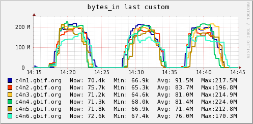
Here we see what we have seen many times - saturating our network.  But why?  These are Mappers that should be hitting local RegionServers using local drives (12 of them).  Looking at the number of data-local mappers spawned, we see that we have very low data-local map tasks:


This is suspicious, and if you see this, start investigating why.  Basically the MR job is spawning tasks to use data that reside on other machines.  For us, that means Mappers that are talking to region servers that are not local to it.  On investigation, and from reading HBASE-1672, we observe that when looking at a task attempt in the MR console, the task attempt and input split locations look suspiciously different:


These actually refer to the same machine, but one is using the IP address, and the other the host name.

HBase is using the TableInputFormat which is returning the IP (thanks Stack for pointing this out).  Now, it is important to note that this code is executed on the client calling machine, as it prepares a job for submission to the cluster.  In my setup I was running over VPN from my laptop which was providing IP addresses for the region locations.  The code in the TableInputFormatBase for our version of HBase was:

String regionLocation = table.getRegionLocation(keys.getFirst()[i]).getServerAddress().getHostname();

But on my laptop, a getHostname() on these machines always returned the IP address.  Moving my code onto the cluster and launching from there solved this issue.

Improvement #2: Ensure HBase is balanced
When starting these tests there were 2 tables on HBase.  HBase reported it was nicely balanced, major table compactions were done.  On running however, we still see a huge bottleneck again shown clearly with bytes_out, bytes_in and region server requests:


Again the network saturation is clear, but 1 region server is getting hammered, and many machines are receiving data.  

Why? Well, we run HBase 0.90 which does balancing across all tables and not on a per table basis.  Thus, while HBase saw it's regions evenly distributed across the servers, one machine was hot spotted for one table.  This is fixed in HBase 0.94, but we don't run that yet and ganglia clearly shows us this is a limitation.  Again, MR is spawning jobs on other machines all hitting one RS and saturating the network.  Fortunately I could delete the unused table and rebalance the lot.

Miscellaneous improvements
Somewhere along the line I saw exceptions reporting timeouts and things like this:

48 Lease exceptions
org.apache.hadoop.hbase.regionserver.LeaseException: org.apache.hadoop.hbase.regionserver.LeaseException: lease '7961909311940960915' does not exist
 at org.apache.hadoop.hbase.regionserver.Leases.removeLease(Leases.java:230)
 at org.apache.hadoop.hbase.regionserver.HRegionServer.next(HRegionServer.java:1879)
 at sun.reflect.GeneratedMethodAccessor15.invoke(Unknown Source)
 at sun.reflect.DelegatingMethodAccessorImpl.invoke(DelegatingMethodAccessorImpl.java:25)
 at java.lang.reflect.Method.invoke(Method.java:597)
 at org.apache.hadoop.hbase.ipc.HBaseRPC$Server.call(HBaseRPC.java:570)
 at org.apache.hadoop.hbase.ipc.HBaseServer$Handler.run(HBaseServer.java:1039)

Basically the HBase client is not reporting to the master quickly enough, and the master kills the client, and thus the task attempt fails.  The result is the JobTracker goes and spawns another task attempt, and here we often observed it was not a map-local attempt - everything we know we need to avoid for performance.  The following were done to address this:

  1. Set the hbase.regionserver.lease.period to 600000, up from 60000.  This was then the same as the TaskTracker timeout, so HBase would timeout the scan client in the same duration that the JobTracker would timeout the Task attempt anyway
  2. Reduce the number of mappers from 44 to 36 on each machine.  Here we just ran a few runs, observed Ganglia load averages etc, repeated with different configuration and ultimately tuned the Mapper count to the point where no exceptions were thrown.  There was no magic recipe to this, other than "rinse and repeat".  This is where Puppet is gold.

The final run
With a balanced HBase environment, and resolving the IP / Host issue, the MR result, and ganglia bytes_in, bytes_out and region server requests are shown:


We still see 5 mappers running across the network, which are due to the FairScheduler deciding it has waited long enough for a data local mapper and spawning another - we might investigate if we want to increase this wait time.

A final thought
All these tests used no Filter in the Scan, thus the entire data was passed from the region server to the mapper.  Adding a filter such as the following, reduces the time to around 90 secs.

      scan.setFilter(new SingleColumnValueFilter(
        "v".getBytes(), 
        "scientific_name".getBytes(), 
        CompareOp.EQUAL,
        "Abies alba".getBytes()));

We are using Hive 0.90 on HBase 0.90 and I believe Hive will push down the "equals" predicates to HBase, which will benefit from these kind of filters.  However, I wanted to run the tests without them, as we will often do range scans, and custom UDFs to do things like point in polygon checking.

Thanks to everyone on the mailing lists for all their support through this.  You all know who you are, but in particular thanks to Lars George and Stack.  All GBIF work is open source, and we are committed to open data - we always welcome collaborations.


Wednesday, 23 May 2012

Hive 0.9 with HBase 0.90

Hive 0.9.0 was released at the beginning of this month and it contains a lot of very nice improvements. Thanks to all involved!

Unfortunately it drops compatibility with HBase 0.90.x due to two issues which introduced a dependency on HBase 0.92:
Fortunately these were relatively easy to revert so that's what we did because we wanted to all the 0.9.0 goodness on our HBase 0.90.4 cluster (CDH3u3).

I've forked Hive on Github and reverted the parts of those two issues (HIVE-2748, HIVE-2764) that were causing problems.

For all those "stuck" with HBase 0.90 (e.g. CDH3 users) we've also deployed this custom Hive HBase Handler to our own Maven repository and will maintain that for the foreseeable future. You can just download the jar file and use it in your projects or use our Maven repository:

  gbif-thirdparty
  http://repository.gbif.org/content/repositories/thirdparty

And then declare a dependency on this custom HBase Handler:

  org.apache.hive
  hive-hbase-handler
  0.9.0
  hbase-0.90-compat

Note for Maven experts: I'm not sure if this is a valid classifier. I couldn't find any naming rules.

That's it! We might maintain this for future versions of Hive but we'd love to hear about any problems in any case.

Tuesday, 20 March 2012

HBase Performance Evaluation continued - The Smoking Gun

Update: See also part 1 and part 3.

In my last post I described my initial foray into testing our HBase cluster performance using the PerformanceEvaluation class.  I wasn't happy with our conclusions, which could largely be summed up as "we're not sure what's wrong, but it seems slow".  So in the grand tradition of people with itches that wouldn't go away, I kept scratching.  Everything that follows is based on testing with PerformanceEvaluation (the jar patched as in the last post) using a 300M row table built with PerformanceEvaluation sequentialWrite 300, and tested with PerformanceEvaluation scan 300.  I ran the scan test 3 times, so you should see 3 distinct bursts of activity in the charts.  And to recap our hardware setup - we have 3 regionservers and a separate master.

The first unsettling ganglia metric that kept me digging was of ethernet bytes_in and bytes_out.  I'll recreate those here:
Figure 1 - bytes_in (MB/s) with single gigabit ethernet
Figure 2 - bytes_out (MB/s) with single gigabit ethernet
This is a single gigabit ethernet link, and that is borne out by the Max values, which are near the theoretical max of 120 megabytes per second (MB/s), and as you can see they certainly aren't sitting at 120 constantly in the way one would expect if ethernet was our bottleneck. But that bytes_in graph sure looks like it's hitting some kind of limit - steep ramp up, relatively constant transfer rate, then steep ramp down.  So I decided to try channel bonding to effectively use 2 gigabit links on each server "bonded" together.  It turns out that's not quite as trivial as it may seem, but in the end I got it working following the Dell/Cloudera configuration suggestion of mode 6 / balance-alb, which is described more in the Linux kernel bonding documentation. The results are shown in the following graphs:

Figure 3 - bytes_in (MB/s) with dual (bonded) gigabit ethernet
Figure 4 - bytes_out (MB/s) with dual (bonded) gigabit ethernet
Unfortunately the scale has changed (ganglia ain't perfect) but you can see we're now hovering a bit higher than the single ethernet case, and at some points swinging significantly above the single ethernet limit (a few gusts up to 150).  So it would seem that even though the single gigabit graphs didn't look like they were hitting theoretical maximum, they were definitely limited.  Not by much though - maybe 10-15%?  As they say, the proof is in the pudding, so what was the final throughput for the two tests?


EthernetThroughput (rows/s)
Single340k
Double357k

Looks like 5%. Certainly not the doubling I was hoping for! Something else must be the limiting factor then, but what?  Well, what does CPU say?
Figure 5 - cpu_idle with dual (bonded) gigabit ethernet
That CPU is saying, "Feed me Seymour!".  If the CPU is hungry, what about the load average?
Figure 6 - one minute load average with dual (bonded) gigabit ethernet
These machines have 8 hyper-threaded cores, so effectively 16 cpus. The load average looks like it's keeping the CPUs fed - hovering around 20. But hang on - the load average isn't all about CPU - it's about work that the whole machine needs to do - including all the io subsystems. So if it ain't network, and it ain't CPU then it's gotta be disks. Let's look at how much time the CPU spent waiting on io (which in this case basically means "waiting on disks"):
Figure 7 - percentage cpu spent in wait_io state, with dual (bonded) gigabit ethernet
From a pure gut perspective, that seems kind of high.  But on closer inspection, that graph also looks familiar - it's basically the same as Figure 6 - the load average. So what can we deduce?  When ethernet is removed as a limiting factor the run queue is filled with processes that all cause an increase in wait_io - which means our processes would all finish faster if they didn't have to wait for io.  The limiting factor must, then, be the disks.

Recap (TL;DR)
Ethernet looked suspiciously capped, but performance (and ethernet usage) only increased slightly when the cap was lifted. Closer inspection of the resulting load average and CPU usage showed that the limiting factor was in fact the disks.  

Solution?  Replacing the disks might help a little - they're 3 year old 2.5" SATA, but they are 7.2k rpm, and a more modern 10k 2.5" would be marginally faster.  The real benefit would probably be more disks - the current wisdom on the mailing lists and in the documentation is to maximize the ratio of disk spindles to cpu cores and I think that's borne out by these results.  In the coming weeks we're going to build a new cluster of 6 machines with 12 disks each and I very much look forward to testing my theories once they're up and running.  Stay tuned!