Faster HBase - hardware matters

As I've written earlier, I've been spending some time evaluating the performance of HBase using PerformanceEvaluation. My earlier conclusions amounted to: bond your network ports and get more disks. So I'm happy to report that we got more disks, in the form of 6 new machines that together make up our new cluster:

Master (c1n4): HDFS NameNode, Hadoop JobTracker, HBase Master, and Zookeeper
Zookeeper (c1n1): Zookeeper for this cluster, master for our other cluster

Slaves (c4n1..c4n6): HDFS DataNode, Hadoop TaskTracker, HBase RegionServer (6 GB heap)

Hardware:
c1n*: 1x Intel Xeon X3363 @ 2.83GHz (quad), 8GB RAM, 2x500G SATA 5.4K
c4n*: Dell R720XD, 2x Intel Xeon E5-2640 @ 2.50GHz (6-core), 64GB RAM, 12x1TB SATA 7.2K


Obviously the new machines come with faster everything and lots more RAM, so first I bonded two ethernet ports and then ran the tests again to see how much we had improved:

Figure 1: Scan performance of new cluster (2x 1gig ethernet)

So, 1 million records/second? Yes, please! That's a performance increase of about 300% over the c2 cluster I tested in my previous posts. Given that we doubled the number of machines and quadrupled the number of drives, that improvement feels about right. But the decline in performance as number of mappers is increased is still a bit suspect - we'd hope that performance would go up with more workers. This is the same behaviour we saw when we were limited by network in our original tests, and ganglia again shows a similar pattern, though this time it looks like we're hitting a limit around the 2 gig ethernet bond:

Figure 2: bytes_in (MB/s) with dual gigabit ethernet

Figure 3: bytes_out (MB/s) with dual gigabit ethernet

Unfortunately our master switch is currently full, so we don't have the extra 6 ports needed to test a triple bond - but given our past experience I feel reasonably confident that it would change Figure 1 such that scan performance increases with number of mappers up to some disk I/O contention limit.

Hang-on, what about data locality?

But there's a bigger question here - why are we using so much network bandwidth in the first place? Why stress about major compactions and data locality when it doesn't seem to get used? Therein lies the rub - PerformanceEvaluation can't take advantage of data locality. Tim wrote about the tremendous importance of TableInputFormat in ensuring maximum scan performance from MapReduce, and PerformanceEvaluation doesn't do that. It assigns a block of ids to scan to different mappers at random, meaning that at best one in six mappers (in our setup) will coincidentally have local data to read, and the rest will all transfer their data across the network. This isn't a bug in PerformanceEvaluation, per se, because it was written to try and emulate the tests that Google ran in their seminal white paper on BigTable, rather than act as a true benchmark for scanning performance. But if you're new to this stuff (as I was) it sure can be confusing. When we switched to scanning our real data using TableInputFormat our throughput jumped to 2M/sec from the 1M/sec we got using PerformanceEvaluation.

Conclusions

While we learned a lot from using PerformanceEvaluation to test our clusters, and it helped to uncover any misconfigurations and taught us how to fine tune lots of parameters, it is not a good tool for benchmarking scan performance. As Tim wrote, scans across our real occurrence data (~370M records) using TableInputFormat are finishing in 3 minutes - for our needs that is excellent and means we're happy with our cluster upgrade. Stay tuned for news about the occurrence download service that Lars and I are writing to take advantage of all this speed :)

Optimizing HBase MapReduce scans (for Hive)

By targeting data locality, full table scans of HBase using MapReduce across 373 million records are reduced from 19 minutes to 2.5 minutes. 

We've been posting some blogs about HBase Performance which are all based on the PerformanceEvaluation tools supplied with HBase.  This has helped us understand many characteristics of our system, but in some ways has sidetracked our tuning - namely investigating channel bonding to help increase inter machine bandwidth believing it was our primary limitation.  While that will help for many things (e.g. the copy between mappers and reducers), a key usage pattern involves full table scans of HBase (spawned by Hive) and in a well setup environment network traffic should be minimal for this.  Here I describe how we approached this problem, and the results.

The environment
We run Ganglia for cluster monitoring (and ours is public) and Puppet to provision machines.  As an aside, without these tools or an equivalent I don't think you can sanely hope to run HBase in production.  Here we are using the 6 node cluster, where each of the 6 slaves run a TaskTracker, DataNode and RegionServer, and each machine is Dell R720xd, with 64GB memory, 12xSATA 1TB drives with dual 6 core hyper threading CPUs.  Quoting the user list: "HBase should be able to stretch its legs with this hardware".

Baseline
As a naive person getting access to the new cluster I started by creating the HBase table, mounted a Hive table on it, and populated it with a select using data from a CSV file.

INSERT OVERWRITE occurrence_hbase SELECT * FROM occurrence_hdfs. 

The first good news was that this ran in only 2.5hrs to load up 367 million records with no pre splitting of the table and no failures (normally we use bulk loading tools but here I was feeling lazy).  I then crafted a super simple MR job based on TableMapReduceUtils that took an unfiltered Scan, and a Mapper that did nothing but increment a counter with the number of rows read.  This is a decent replica of what Hive would do when doing a range query (Hive does not do predicate push down to HBase with filters except for equality filters at the moment).  The first run took 19 minutes.  This test was across 200GB data (uncompressed) spread across 84 hard drives and 72 hyper threading cores reading it, so I knew it was too slow.  We started digging... here you find some insights as to how we approached the task.

Improvement #1: Host name versus IP address
On an early run, we see the following on the Ganglia bytes_out:

Here we see what we have seen many times - saturating our network.  But why?  These are Mappers that should be hitting local RegionServers using local drives (12 of them).  Looking at the number of data-local mappers spawned, we see that we have very low data-local map tasks:

This is suspicious, and if you see this, start investigating why.  Basically the MR job is spawning tasks to use data that reside on other machines.  For us, that means Mappers that are talking to region servers that are not local to it.  On investigation, and from reading HBASE-1672, we observe that when looking at a task attempt in the MR console, the task attempt and input split locations look suspiciously different:

These actually refer to the same machine, but one is using the IP address, and the other the host name.

HBase is using the TableInputFormat which is returning the IP (thanks Stack for pointing this out).  Now, it is important to note that this code is executed on the client calling machine, as it prepares a job for submission to the cluster.  In my setup I was running over VPN from my laptop which was providing IP addresses for the region locations.  The code in the TableInputFormatBase for our version of HBase was:

String regionLocation = table.getRegionLocation(keys.getFirst()[i]).getServerAddress().getHostname();

But on my laptop, a getHostname() on these machines always returned the IP address.  Moving my code onto the cluster and launching from there solved this issue.

Improvement #2: Ensure HBase is balanced
When starting these tests there were 2 tables on HBase.  HBase reported it was nicely balanced, major table compactions were done.  On running however, we still see a huge bottleneck again shown clearly with bytes_out, bytes_in and region server requests:

Again the network saturation is clear, but 1 region server is getting hammered, and many machines are receiving data.  

Why? Well, we run HBase 0.90 which does balancing across all tables and not on a per table basis.  Thus, while HBase saw it's regions evenly distributed across the servers, one machine was hot spotted for one table.  This is fixed in HBase 0.94, but we don't run that yet and ganglia clearly shows us this is a limitation.  Again, MR is spawning jobs on other machines all hitting one RS and saturating the network.  Fortunately I could delete the unused table and rebalance the lot.

Miscellaneous improvements
Somewhere along the line I saw exceptions reporting timeouts and things like this:

48 Lease exceptions
org.apache.hadoop.hbase.regionserver.LeaseException: org.apache.hadoop.hbase.regionserver.LeaseException: lease '7961909311940960915' does not exist
 at org.apache.hadoop.hbase.regionserver.Leases.removeLease(Leases.java:230)
 at org.apache.hadoop.hbase.regionserver.HRegionServer.next(HRegionServer.java:1879)
 at sun.reflect.GeneratedMethodAccessor15.invoke(Unknown Source)
 at sun.reflect.DelegatingMethodAccessorImpl.invoke(DelegatingMethodAccessorImpl.java:25)
 at java.lang.reflect.Method.invoke(Method.java:597)
 at org.apache.hadoop.hbase.ipc.HBaseRPC$Server.call(HBaseRPC.java:570)
 at org.apache.hadoop.hbase.ipc.HBaseServer$Handler.run(HBaseServer.java:1039)

Basically the HBase client is not reporting to the master quickly enough, and the master kills the client, and thus the task attempt fails.  The result is the JobTracker goes and spawns another task attempt, and here we often observed it was not a map-local attempt - everything we know we need to avoid for performance.  The following were done to address this:

1. Set the hbase.regionserver.lease.period to 600000, up from 60000.  This was then the same as the TaskTracker timeout, so HBase would timeout the scan client in the same duration that the JobTracker would timeout the Task attempt anyway
2. Reduce the number of mappers from 44 to 36 on each machine.  Here we just ran a few runs, observed Ganglia load averages etc, repeated with different configuration and ultimately tuned the Mapper count to the point where no exceptions were thrown.  There was no magic recipe to this, other than "rinse and repeat".  This is where Puppet is gold.

The final run
With a balanced HBase environment, and resolving the IP / Host issue, the MR result, and ganglia bytes_in, bytes_out and region server requests are shown:

We still see 5 mappers running across the network, which are due to the FairScheduler deciding it has waited long enough for a data local mapper and spawning another - we might investigate if we want to increase this wait time.

A final thought
All these tests used no Filter in the Scan, thus the entire data was passed from the region server to the mapper.  Adding a filter such as the following, reduces the time to around 90 secs.

      scan.setFilter(new SingleColumnValueFilter(
        "v".getBytes(), 
        "scientific_name".getBytes(), 
        CompareOp.EQUAL,
        "Abies alba".getBytes()));

We are using Hive 0.90 on HBase 0.90 and I believe Hive will push down the "equals" predicates to HBase, which will benefit from these kind of filters.  However, I wanted to run the tests without them, as we will often do range scans, and custom UDFs to do things like point in polygon checking.

Thanks to everyone on the mailing lists for all their support through this.  You all know who you are, but in particular thanks to Lars George and Stack.  All GBIF work is open source, and we are committed to open data - we always welcome collaborations.

Hive 0.9 with HBase 0.90

Hive 0.9.0 was released at the beginning of this month and it contains a lot of very nice improvements. Thanks to all involved!

Unfortunately it drops compatibility with HBase 0.90.x due to two issues which introduced a dependency on HBase 0.92:

• https://issues.apache.org/jira/browse/HIVE-2748
• https://issues.apache.org/jira/browse/HIVE-2764

Fortunately these were relatively easy to revert so that's what we did because we wanted to all the 0.9.0 goodness on our HBase 0.90.4 cluster (CDH3u3).

I've forked Hive on Github and reverted the parts of those two issues (HIVE-2748, HIVE-2764) that were causing problems.

For all those "stuck" with HBase 0.90 (e.g. CDH3 users) we've also deployed this custom Hive HBase Handler to our own Maven repository and will maintain that for the foreseeable future. You can just download the jar file and use it in your projects or use our Maven repository:

  gbif-thirdparty
  http://repository.gbif.org/content/repositories/thirdparty

And then declare a dependency on this custom HBase Handler:

  org.apache.hive
  hive-hbase-handler
  0.9.0
  hbase-0.90-compat

Note for Maven experts: I'm not sure if this is a valid classifier. I couldn't find any naming rules.

That's it! We might maintain this for future versions of Hive but we'd love to hear about any problems in any case.

HBase Performance Evaluation continued - The Smoking Gun

Update: See also part 1 and part 3.

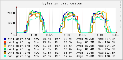
In my last post I described my initial foray into testing our HBase cluster performance using the PerformanceEvaluation class.  I wasn't happy with our conclusions, which could largely be summed up as "we're not sure what's wrong, but it seems slow".  So in the grand tradition of people with itches that wouldn't go away, I kept scratching.  Everything that follows is based on testing with PerformanceEvaluation (the jar patched as in the last post) using a 300M row table built with PerformanceEvaluation sequentialWrite 300, and tested with PerformanceEvaluation scan 300.  I ran the scan test 3 times, so you should see 3 distinct bursts of activity in the charts.  And to recap our hardware setup - we have 3 regionservers and a separate master.

The first unsettling ganglia metric that kept me digging was of ethernet bytes_in and bytes_out.  I'll recreate those here:

Figure 1 - bytes_in (MB/s) with single gigabit ethernet

Figure 2 - bytes_out (MB/s) with single gigabit ethernet

This is a single gigabit ethernet link, and that is borne out by the Max values, which are near the theoretical max of 120 megabytes per second (MB/s), and as you can see they certainly aren't sitting at 120 constantly in the way one would expect if ethernet was our bottleneck. But that bytes_in graph sure looks like it's hitting some kind of limit - steep ramp up, relatively constant transfer rate, then steep ramp down.  So I decided to try channel bonding to effectively use 2 gigabit links on each server "bonded" together.  It turns out that's not quite as trivial as it may seem, but in the end I got it working following the Dell/Cloudera configuration suggestion of mode 6 / balance-alb, which is described more in the Linux kernel bonding documentation. The results are shown in the following graphs:

Figure 3 - bytes_in (MB/s) with dual (bonded) gigabit ethernet

Figure 4 - bytes_out (MB/s) with dual (bonded) gigabit ethernet

Unfortunately the scale has changed (ganglia ain't perfect) but you can see we're now hovering a bit higher than the single ethernet case, and at some points swinging significantly above the single ethernet limit (a few gusts up to 150).  So it would seem that even though the single gigabit graphs didn't look like they were hitting theoretical maximum, they were definitely limited.  Not by much though - maybe 10-15%?  As they say, the proof is in the pudding, so what was the final throughput for the two tests?

Ethernet	Throughput (rows/s)
Single	340k
Double	357k

Looks like 5%. Certainly not the doubling I was hoping for! Something else must be the limiting factor then, but what?  Well, what does CPU say?

Figure 5 - cpu_idle with dual (bonded) gigabit ethernet

That CPU is saying, "Feed me Seymour!".  If the CPU is hungry, what about the load average?

Figure 6 - one minute load average with dual (bonded) gigabit ethernet

These machines have 8 hyper-threaded cores, so effectively 16 cpus. The load average looks like it's keeping the CPUs fed - hovering around 20. But hang on - the load average isn't all about CPU - it's about work that the whole machine needs to do - including all the io subsystems. So if it ain't network, and it ain't CPU then it's gotta be disks. Let's look at how much time the CPU spent waiting on io (which in this case basically means "waiting on disks"):

Figure 7 - percentage cpu spent in wait_io state, with dual (bonded) gigabit ethernet

From a pure gut perspective, that seems kind of high.  But on closer inspection, that graph also looks familiar - it's basically the same as Figure 6 - the load average. So what can we deduce?  When ethernet is removed as a limiting factor the run queue is filled with processes that all cause an increase in wait_io - which means our processes would all finish faster if they didn't have to wait for io.  The limiting factor must, then, be the disks.

Recap (TL;DR)

Ethernet looked suspiciously capped, but performance (and ethernet usage) only increased slightly when the cap was lifted. Closer inspection of the resulting load average and CPU usage showed that the limiting factor was in fact the disks.  

Solution?  Replacing the disks might help a little - they're 3 year old 2.5" SATA, but they are 7.2k rpm, and a more modern 10k 2.5" would be marginally faster.  The real benefit would probably be more disks - the current wisdom on the mailing lists and in the documentation is to maximize the ratio of disk spindles to cpu cores and I think that's borne out by these results.  In the coming weeks we're going to build a new cluster of 6 machines with 12 disks each and I very much look forward to testing my theories once they're up and running.  Stay tuned!

Performance Evaluation of HBase

Update: See also followup posts: part 2 and part 3.

In the last post Lars talked about setting up Ganglia for monitoring our Hadoop and HBase installations.  That was in preparation for giving HBase a solid testing run to assess its suitability for hosting our index of occurrence records.  One of the important features in our new Data Portal will be the "Download" function that lets people download occurrences matching some search criteria and currently that process is a very manual and labour intensive one, so automating it will be a big help to us.  Using HBase it would be implemented as a full table scan, and that's why I've spent some time testing our scan performance. Anyone who has been down this road will probably have encountered the myriad opinions on what will improve performance (some of them conflicting) along with the seemingly endless parameters that can be tuned in a given cluster.  The overall result of that kind of research is: "You gotta do it yourself".  So here we go.

Because we hope to get some feedback from the HBase community on our results (ideally comparisons to other running clusters) we decided to use the PerformanceEvaluation class that ships with HBase.  Unfortunately it's not completely bug free so I've had to patch it to work in the way we would like.  From a stock cdh3u3 HBase I patched HBASE-5401 and HBASE-4688, and had a good, hard think about HBASE-5402.  There are a bunch of things I learned about the PerformanceEvaluation (PE) class in the last few weeks, and the implications of 5402 are some of them.  If anyone's interested I'll blog about those another time, but for now suffice it to say that in my final suite of tests I went with writing tables using "sequentialWrite" (which obviates the difficulties in 5402) and doing scans with the "scan" test.

There are many variables that can be changed in an HBase/Hadoop cluster setup but you have to start somewhere so here's our basic config that remained unchanged throughout the test (you can see more at its ganglia page):

Master (c1n2): HDFS NameNode, Hadoop JobTracker, HBase Master, and Zookeeper
Slaves (c2n1, c2n2, c2n3): HDFS DataNode, Hadoop TaskTracker, HBase RegionServer (6 GB heap)

Hardware:
c1n2: 1x Intel(R) Xeon(R) X3363 @ 2.83GHz (quad), 8GB RAM, 2x500G SATA 5.4K
c2n*: 2x Intel(R) Xeon(R) E5630 @ 2.53GHz (quad), 24GB RAM, 6x250G SATA 7.2K

The parameters I varied are:

• number of rows in the test table (50M, 100M, 200M)
• number of mappers per server (8, 10, 12, 14, 20 - more than 20 and we ran out of RAM)
• snappy compression (on/off)
• scanner caching (size)
• block caching (on/off)

Test Methodology

The test methodology was to start with an empty HDFS (replication factor of 2), an empty HBase and no other tasks running on the machines.  Then build a table using a command line like 

hbase org.apache.hadoop.hbase.PerformanceEvaluation sequentialWrite 100

and then wait for the split/compaction cycle to complete, and then run a major compaction to encourage data locality.  In tests using compression I would construct an empty table by hand, specifying compression=>'SNAPPY' for the info column family before running the sequentialWrite. I'd also wait for the region balancer to run, ensuring that all regionservers had an equal number of regions (+/- 1). Once that was complete I would run a scan test with a command like:

hbase org.apache.hadoop.hbase.PerformanceEvaluation scan 100

and note the real time taken as reported by the JobTracker as well as the total time spent in mappers as reported by PE itself.  I ran each scan test 3 times unless the first 2 tests were very close, in which case I sometimes skipped the 3rd run. Note also that PE uses 10 byte keys and 1000 kilobyte values by default. 

Two things were immediately obvious in my caching tests, which I'll talk about briefly before getting into the results proper.

Scanner Caching

The HBase API Scan class takes a setting called setCaching(int caching) which tells the scanner how many rows to fetch at a time from the server.  This defaults to 1, which is optimal for single gets, but is decidedly suboptimal for big scans like ours. Unfortunately PE doesn't allow for explicitly setting this value on the command line and so I took the advice of the API Javadoc and passed in a value of 1000 for the property hbase.client.scanner.caching in the hbase-site.xml file that forms the configuration for the MapReduce job that is PE.  It would seem, though, that this property is not being honoured by HBase and so my initial tests all ran with a cache size of 1, producing poor results.  I subsequently hard-coded the setCaching(1000) on the scans themselves in the PE and saw significant improvements. Those differences are visible in the results, below.

Block Caching

When I say block caching I mean HBase blocks - not HDFS blocks.  See the HBase guide or Lars George's excellent HBase: The Definitive Guide for many more details. You'll see many recommendations from different sources to turn block caching off during scans but it's not immediately obvious why that should be.  It turns out that it has no performance implications for the scan itself, but will significantly impact any random reads (gets) that may be relying on recently loaded blocks.  If the scan is using the block cache then it will load the cache with a block, read the block, and then load the next one, ignoring the first one for the rest of the scan.  The earlier loaded blocks will be evicted quickly (as new blocks are loaded) leading to "cache churn".  So I tested the block cache on and off and concluded that there was no difference in a dedicated scan test (no other activity in the cluster) and so for the rest of my tests I left the block cache on.  In order to test this behaviour I again had to hard-code PE with setCacheBlocks(false) (it defaults to true).

The Results

The full spreadsheet is available for download from our google code site.  I've just included the summary chart here, because it pretty much tells the story.  Of note: the y-axis is Records / second which I calculate as the total records scanned divided by the total time for the job as reported by the JobTracker.  This doesn't, therefore, take any of the PE generated per-mapper counts/times into account (which are still somewhat mysterious to me).

Conclusions (within our obviously limited test environment):

• with bigger datasets, more mappers are better; with smaller datasets, somewhat fewer are better
• compression slows things down.  This is probably the most surprising (and contentious) finding.  We would expect performance to improve with compression (at worst staying the same) because there is much less data to transfer when the files are compressed, and I/O is typically the limiting factor in HBase performance.  I kept an eye on the cpus with ganglia during the uncompressed tests and sure enough, they spent approximately double the amount of time in io_wait as in the compressed tests.
• ganglia revealed no obvious bottlenecks during the scan.  You can look at our ganglia charts from the past few weeks and apart from a few purposefully degenerate tests there was no obvious component that was limiting things - cpus never went above 60% (io_wait never above 30%), and RAM and disks "looked ok".  If anyone has insight here we'd really appreciate it.
• total variability across all these tests was only about 20%.  Either all tests are hitting the same, as yet unseen, hardware or configuration limit, or there really is no silver bullet to performance increases - tuning is an incremental thing.
• there are still strange things going on :)  I can't explain the fact that in the compressed test performance increases from 50 to 100M records, and then decreases dramatically with 200M records.

We'd love feedback on these results, both in terms of how we can improve our testing and in interpreting the results, as well as any numbers you may have from your clusters when running PE.  Is 300k records per second even in the ballpark?  It's crazy that these data don't exist out there already, so hopefully this post helps alleviate that somewhat.  

The good news is that we'll be getting new cluster hardware soon, and then I think the next step is to load our real occurrences data into a table and run similar scanning tests against it to optimize those scans.  Of course then we'll start writing new records at the same time, and then things will get.... interesting.  Should be fun :)

Monitoring Hadoop and HBase

We're getting serious in our Hadoop adoption. The first process (our so called "rollover") is now in production and it uses Hadoop, Hive, Oozie and various other parts of the Hadoop ecosystem.

Our next step is evaluating HBase and its performance on our (small and aging) cluster. To do that properly and to fix a rather embarrassing situation we first had to get proper monitoring up and running for our cluster. So far we've only had Cacti stats for OS level things (CPU, I/O, etc.) but we were missing actual Hadoop statistics.

So we've now set up Ganglia at GBIF and the best news is it's public and using the very latest Ganglia 3.3 which was released only a few days ago in February 2012. The setup was relatively painless. Ganglia was just nice to work with. To get monitoring of HBase working we had to apply HBASE-4854 because it's not included in our Hadoop distribution (CDH3u2). Thanks to Lars George for the hint.

So we can happily report that Ganglia 3.3 works perfect with the GangliaContext31 from Hadoop.

Now all that's left is learning what most of these stats mean and then trying to extract useful information from them. Any hints are more than welcome and the HBase community already offered to help. Thank you very much!

For anyone interested in a few notes and details about how we set Ganglia up keep on reading.

BioCASe now producing DarwinCore Archives

Guest post from Jörg Holetschek, Botanic Garden and Botanical Museum Berlin-Dahlem.

The traditional way of sharing occurrence data with GBIF has been web-service-based for years. Data publishers have used one of the existing provider software packages (DiGIR, BioCASe or TAPIR Link) to expose their data as a DiGIR-, BioCASe- or TAPIR-compliant web service. Biodiversity networks such as GBIF used harvesters to crawl and index the records published by these services, an approach that works fine for small and medium-sized datasets, but runs into difficulties when record numbers hit the millions: Harvesting can take days and puts a heavy load on both the publisher and the crawler.

To overcome this, GBIF recently introduced DarwinCore Archives for storing all information of a dataset to be published in a single file. GBIF directly ingesting this file eliminates the time-consuming back-and-forth communication between data provider and harvester, speeding up the process and reducing load for both sides. GBIF’s IPT allows easy creation of such DarwinCore Archives and is a good option for providers that have already used the DarwinCore standard in the past or that want to share rather slim observation data.

However, sixty-two of GBIF’s data publishers are currently using BioCASe. In contrast to DarwinCore, BioCASe and its associated data standard ABCD are targeted mainly at rich data originating from specimens of natural history collections (even though it can be used for any type of occurrence data, including observations). Many of the BioCASe data providers also share their data with special interest networks such as GeoCASe, the DNA-Bank Network, or the EDIT Specimen network, all of them relying on BioCASe web services. Switching to the IPT and the associated DarwinCore standard is not an option for them.

For this reason, we decided to extend the BioCASe Provider Software with a feature to create DarwinCore Archives. This allows providers to continue using the rich ABCD schema (or one of its extensions) for the specific networks they’re connected to while using DarwinCore Archives to share their data with GBIF. In order to combine the richness of ABCD with the efficiency of downloadable archives, we created a hybrid in-between, the so called ABCD Archives, which can be used instead of the BioCASe web service for harvesting purposes (see figure below).

The first step – creating the ABCD archive – is implemented natively in the Provider Software in Python. The second step – transforming the ABCD archive into one or several DarwinCore archives – is done by Pentaho Data Transformation, an open source library also known as Kettle. In the current version 3.0, the transformation step is a stand-alone command-line application that can be downloaded separately; ultimately, it will be bundled with the Provider Software and integrated into the user interface.

The latest version of the Provider Software and the DarwinCore Creator can be downloaded from the BioCASe website. A detailed documentation of the new archiving features can be found in the PyWrapper Wiki. The wiki also stores a sample ABCD archive and a sample DarwinCore archive created by BioCASe.